Class 11 Causal Inference & Potential Outcome Framework
1 Causal Inference
1.1 Our Journey So Far
Any business activity brings benefits and costs. We’re given the benefit information in all the case studies so far
Apple (Week 1): influencer marketing increases sales by 2.5%
1st assignment: loyalty programme increases retention rate to 95%
In reality, this benefit information is often not readily available, and it’s our job as data scientists to correctly measure them using causal inference tools.
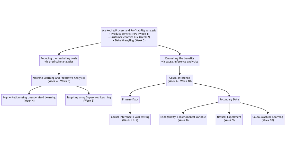
1.2 Causal Inference Road Map
1.3 Learning Objectives
Understand key concepts of causal inference
- Rubin’s potential outcome framework
- Fundamental problem of causal inference
- Average treatment effect (ATE) and randomisation
Learn the steps to conduct randomised controlled trials (RCTs)
1.4 Why Causal Inference Matters? Example 1
Tom purchases paid ads on Instagram to advertise his new bubble tea shop. Instagram ads are targeted to individuals who are predicted to have a higher likelihood of being bubble tea lovers. In the end, some Instagram users saw no ads and some saw the ads. The purchase rates for each group are shown below.

Question: Can Tom be confident in concluding that the Instagram ads are effective in converting new customers?
1.5 Why Causal Inference Matters? Example 2
Tom bought marketing survey data from a consulting agency. The survey collected prices and store visits (sales) for different bubble tea shops in Canary Wharf. Tom finds that there seems to be a positive relationship between prices and store visits.

Question: Can Tom conclude that he should also increase the prices for his bubble tea shop to increase the store visits?
1.6 Why Causal Inference Matters? Example 3
This is a fighter plane that just returned from the battlefield. Red dots are bullet holes.
Which part of A, B, and C would you reinforce to increase the pilot’s survival rate?

1.7 Why Causal Inference Matters? Example 4
I have kept a secret from you for a long time. It’s time for me to confess…
1.8 Nobel Prize in Economics (2021)

[…] the other half jointly to Joshua D. Angrist and Guido W. Imbens “for their methodological contributions to the analysis of causal relationships.”
1.9 Causal Inference
Causal inference is the process of estimating the unbiased causal effects of a particular policy/business intervention on the outcome variables of interest.
Correlation != Causation: Machine learning models are good at finding correlations, but not causation. For example, on rainy days, we observe more umbrellas on the street
correct correlation statement: number of umbrellas is positively correlated with rainfall
correct causal statement: heavier rain leads to more umbrellas
incorrect causal statement: more umbrellas lead to heavier rain
Causality becomes more complex in the business world. Managers can easily make mistakes without causal inference training.
- Imagine if the actual causal effect of Instagram ads on incremental profit per customer is £1 for Tom, and Tom pays £1.5 for each click
2 Potential Outcome Framework
2.1 Rubin Causal Model and the Potential Outcome Framework
The Rubin causal model (RCM), or the Potential Outcome Framework, is the well-accepted framework for thinking about causal effects.
For each customer \(i\), we can define the potential outcomes in order to evaluate the causal effect of a treatment on their outcomes:
\(Y^{1}_i\): the outcome if the customer is exposed to the treatment, ceteris paribus
\(Y^{0}_i\): the outcome if the customer is not exposed to the treatment, ceteris paribus
Important
Potential outcomes are independent of reality. They are not the same as the observed outcomes in reality.
2.2 The Stable Unit Treatment Value Assumption (SUTVA)
For the potential outcomes to be well-defined, we need an important assumption called the Stable Unit Treatment Value Assumption (SUTVA). SUTVA has two parts:
- No interference: The potential outcomes for any unit do not vary with the treatments assigned to other units.
- Example violation: In an advertising campaign, if a treated customer tells their friends (who are in the control group) about the product, this could influence the friends’ purchasing behavior, violating the no-interference assumption.
- Consistency: The treatment is the same for all units in the treatment group.
- Example violation: If “receiving an ad” involves some customers seeing a video ad and others seeing a banner ad, the treatment has hidden variations, violating the consistency assumption.
Note
SUTVA is a crucial assumption for most causal inference methods. When designing A/B tests, it’s important to consider whether SUTVA is likely to hold.
2.3 Definition: Individual Treatment Effects
- The causal effect of the treatment on the individual \(i\) is the difference between the two potential outcomes. We define the individual treatment effect \(\delta_i\) as follows
\[ \delta_i = Y^1_i - Y^0_i \]
2.4 Example
Tom would like to measure the causal effect of seeing a displayed ad on customer purchase intention.
- Treatment: customer \(i\) seeing a display ad
- Control: customer \(i\) not seeing a display ad
2.5 Examples of Individual Treatment Effects
Let’s imagine we have retrieved all infinity stones from Thanos, and have created a parallel universe, in addition to our own universe.
In Our Universe, Dr strange sees a display ad for bubble tea, while in the Parallel Universe, he does not see the ad.
In Our Universe, with a displayed ad
- Dr Strange has a purchase intention of 70%
In Parallel Universe, without a displayed ad
- Dr Strange has a purchase intention of 60%
| Customer | Y1 | Y0 | Effect | Treated.in.Our.Universe. |
|---|---|---|---|---|
| Dr Strange | 0.7 | 0.6 | 0.1 | Yes |
2.6 A Motivating Example: A Group of Customers
- Conceptually, we can collect a sample of customers, and estimate individual treatment effect for each of them
| Customer | Y1 | Y0 | Effect | Treated.in.Our.Universe. |
|---|---|---|---|---|
| Dr Strange | 0.70 | 0.60 | 0.10 | Yes |
| Iron Man | 0.55 | 0.50 | 0.05 | No |
| Thor | 0.80 | 0.72 | 0.08 | No |
| Hulk | 0.60 | 0.62 | -0.02 | Yes |
- To summarise, to measure the individual treatment effect of the ads on a customer’s purchase intention, we need to observe both potential outcomes of the same individual in parallel universes (i.e., with and without being exposed to the treatment).
2.7 Notations for Reality and Realised Outcomes
So far, we have only talked about potential outcomes in parallel universes. Now, let’s introduce some notations for realised outcomes (i.e., what we observe in Our Universe, the real world for each individual customer).
We define a binary variable \(D_i\) to denote whether customer \(i\) is treated or not in reality.
We use \(D_i = 1\) to denote the treatment group in reality.
We use \(D_i = 0\) to denote the control group in reality.
2.8 Fundamental Problem of Causal Inference: Realised Outcomes
We can observe ONLY ONE potential outcome in our reality, depending on whether the customer is treated or not.
If a customer sees a display ad in reality, we only observe their potential outcome when being treated \(Y^1\), i.e., \(Y^1_i|D_i = 1\)
- However, we never observe the other potential outcome when being untreated: \(Y^0_i|D_i = 1\)
If a customer does not see a display ad in reality, we only observe their potential outcome when being untreated \(Y^0\), i.e., \(Y^0_i|D_i = 0\)
- However, we never observe the other potential outcome when being treated: \(Y^1_i|D_i = 0\)
In other words, the other potential outcome, i.e., counterfactual outcomes, are never observed in our reality
2.9 Numeric Example
In the previous table, Dr Strange and Hulk are treated in our reality, while Iron Man and Thor are not treated.
Then, for Dr Strange, our notations would be as follows:
- Realised outcome: \(Y^1_i |D_i = 1 = 0.7\) (We only observe this potential outcome in our reality)
- Counterfactual outcome: \(Y^0_i |D_i = 1 = 0.6\) (We never observe this potential outcome in our reality)
| Customer | Y1 | Y0 | Treated |
|---|---|---|---|
| Dr Strange | 0.7 | ? | Yes |
| Iron Man | ? | 0.5 | No |
| Thor | ? | 0.72 | No |
| Hulk | 0.6 | ? | Yes |
2.10 Fundamental Problem of Causal Inference
- Since it is impossible to see both potential outcomes at once, one of the potential outcomes is always missing, we can never quantify the individual-level treatment effects. This dilemma is called the Fundamental Problem of Causal Inference.
| subject | Treated | Y1 | Y0 | Y1-Y0 |
|---|---|---|---|---|
| Dr Strange | Yes | 0.7 | ? | ? |
| Iron Man | No | ? | 0.5 | ? |
| Thor | No | ? | 0.72 | ? |
| Hulk | Yes | 0.6 | ? | ? |
3 Average Treatment Effects
3.1 The Average Treatment Effect (ATE)
- Since individual treatment effects are unobservable, we often care more about the average treatment effects (ATE) on the population level. The ATE is defined as the average of individual treatment effects across the population.
\[ ATE = E[Y^1_i - Y^0_i] = \frac{1}{N} \sum_{i=1}^{N} (Y^1_i - Y^0_i) \]
3.2 Obtain the Average Treatment Effect through Randomisation
To quantify the correct ATE, we must randomise who receives the treatment, instead of targeting or letting the individuals choose the treatment.
After randomisation, we can then obtain the ATE by comparing the difference in the average outcomes across the treatment group and control group. Because randomisation ensures that
Selection bias is fully removed1
The treatment effects on the treatment group individuals and the control group individuals should be equal. The former is called the average treatment effects on the treated (ATT), and the latter is called the average treatment effects on the untreated (ATU).
3.3 Gold Standard of Causal Inference
- Mathematically, the previous slide can be represented by the Basic Identity of Causal Inference:
\[\begin{align*} & E[Y^1|D_i = 1] - E[Y^0|D_i = 0] \\ & = E[Y^1|D_i = 1] - E[Y^0|D_i = 1] \\ &+ E[Y^0|D_i = 1] - E[Y^0|D_i = 0] \end{align*}\]

- Randomised experiments makes ATT equal to ATE, and removes selection bias. Thus, randomised experiments are the gold standard of causal inference.
Footnotes
Selection bias refers to the pre-existing difference between the treatment group and control group even without the treatment↩︎