Class 7 Unsupervised Learning and K-Means Clustering
1 Overview of Predictive Analytics
1.1 Learning Objectives for Today
Understand the concept of unsupervised learning
Understand how to apply K-means clustering and determine the optimal number of clusters
How to apply clustering analysis to customer segmentation for M&S
1.2 Roadmap for Predictive Analytics
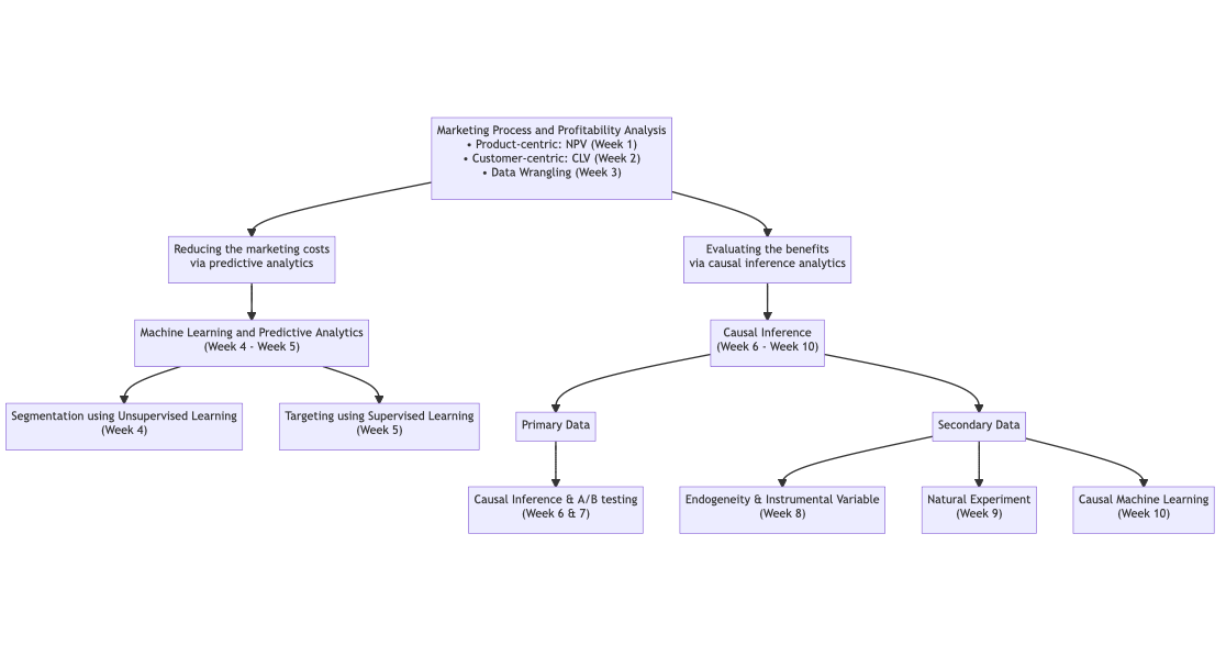
In Weeks 4 and 5, we will learn how to utilise machine learning and predictive analytics to improve ROI for M&S.
We will learn two types of predictive analytics models:
Unsupervised learning (Week 4): K-means clustering for customer segmentation, and then target the most responsive customer segments
Supervised learning (Week 5): Decision trees and Random Forest for individualised customer targeting
1.3 Types of Predictive Analytics
Unsupervised Learning
- Only observe X => want to uncover unknown subgroups
Supervised Learning
- Observe both X and Y => want to predict Y for new data
In Term 2, you will learn predictive analytics models systematically (Machine Learning). By then, think about how those techniques can be applied to these case studies.
1.4 Types of Predictive Analytics

(Reinforcement learning is beyond the scope of this course, but at the high level, it involves learning optimal actions through trial and error to maximize cumulative rewards.)
2 K-Means Clustering
2.1 K-Means Clustering
K-means clustering is one of the most commonly used unsupervised machine learning algorithms for partitioning a given data set into a set of k groups (i.e. k clusters), where k represents the number of groups pre-specified by the analyst.
For data scientists, it can classify customers into multiple segments (i.e., clusters), such that customers within the same cluster are as similar as possible, whereas customers from different clusters are as dissimilar as possible.
Input: (1) customer characteristics; (2) the number of clusters
Output: cluster membership of each customer
2.2 Similarity and Dissimilarity
The clustering of observations into groups requires computing the (dis)similarity between each pair of observations. The result of this computation is known as a dissimilarity or distance matrix.
The choice of similarity measures is a critical step in clustering.
The most common distance measures are the Euclidean distance (the default for K-means).
2.3 Euclidean Distance
The most common distance measure in machine learning is the Euclidean distance. In the following equation, we define the Euclidean distance between two customers (x) and (y) in an n-dimensional space (i.e., n different characteristics) as: \[ d_{\text{euc}}(x, y) = \sqrt{\sum_{i=1}^{n} (x_i - y_i)^2} \]
Example of Income and Spending for 3 customers
- \(Customer \space 1\) =>
c("income"=5, "spending"=3) - \(Customer \space 2\) =>
c("income"=10, "spending"=4) - \(Customer \space 3\) =>
c("income"=20, "spending"=12)
- \(Customer \space 1\) =>
Euclidean distance
- \(d_{\text{euc}}(2, 1) = \sqrt{(10-5)^2 + (4-3)^2} = \sqrt{25 + 1} = \sqrt{26}\)
- \(d_{\text{euc}}(2, 3) = \sqrt{(10-20)^2 + (4-12)^2} = \sqrt{100 + 64} = \sqrt{164}\)
Code
Income <- c(5, 10, 20)

Spending <- c(3, 4, 12)

data <- data.frame(Income, Spending, ID = c("Customer 1", "Customer 2", "Customer 3"))

ggplot(data, aes(x = Income, y = Spending)) +
    geom_point(aes(shape = ID, color = ID), size = 2.5) +
    geom_text(aes(label = rownames(data)), vjust = -0.5) +
    theme_stata()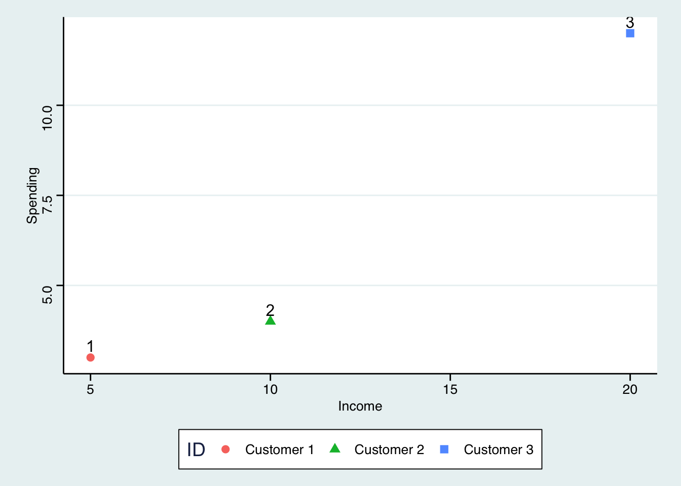
Code
Income <- c(5, 10, 20)

Spending <- c(3, 4, 12)

data <- data.frame(Income, Spending, ID = c("Customer 1", "Customer 2", "Customer 3"))

ggplot(data, aes(x = Income, y = Spending)) +
    geom_point(aes(shape = ID, color = ID), size = 2.5) +
    geom_text(aes(label = rownames(data)), vjust = -0.5) +
    theme_stata() +
    # show the Euclidean distance between Customer 1 and Customer 2; also show the vertical and horizontal lines
    geom_segment(aes(x = 5, y = 3, xend = 10, yend = 4), linetype = "dashed") +
    geom_segment(aes(x = 5, y = 3, xend = 5, yend = 4), linetype = "dashed") +
    geom_segment(aes(x = 5, y = 4, xend = 10, yend = 4), linetype = "dashed") +

    # show the Euclidean distance between Customer 2 and Customer 3; also show the vertical and horizontal lines
    geom_segment(aes(x = 10, y = 4, xend = 20, yend = 12), linetype = "dashed") +
    geom_segment(aes(x = 10, y = 4, xend = 10, yend = 12), linetype = "dashed") +
    geom_segment(aes(x = 10, y = 12, xend = 20, yend = 12), linetype = "dashed")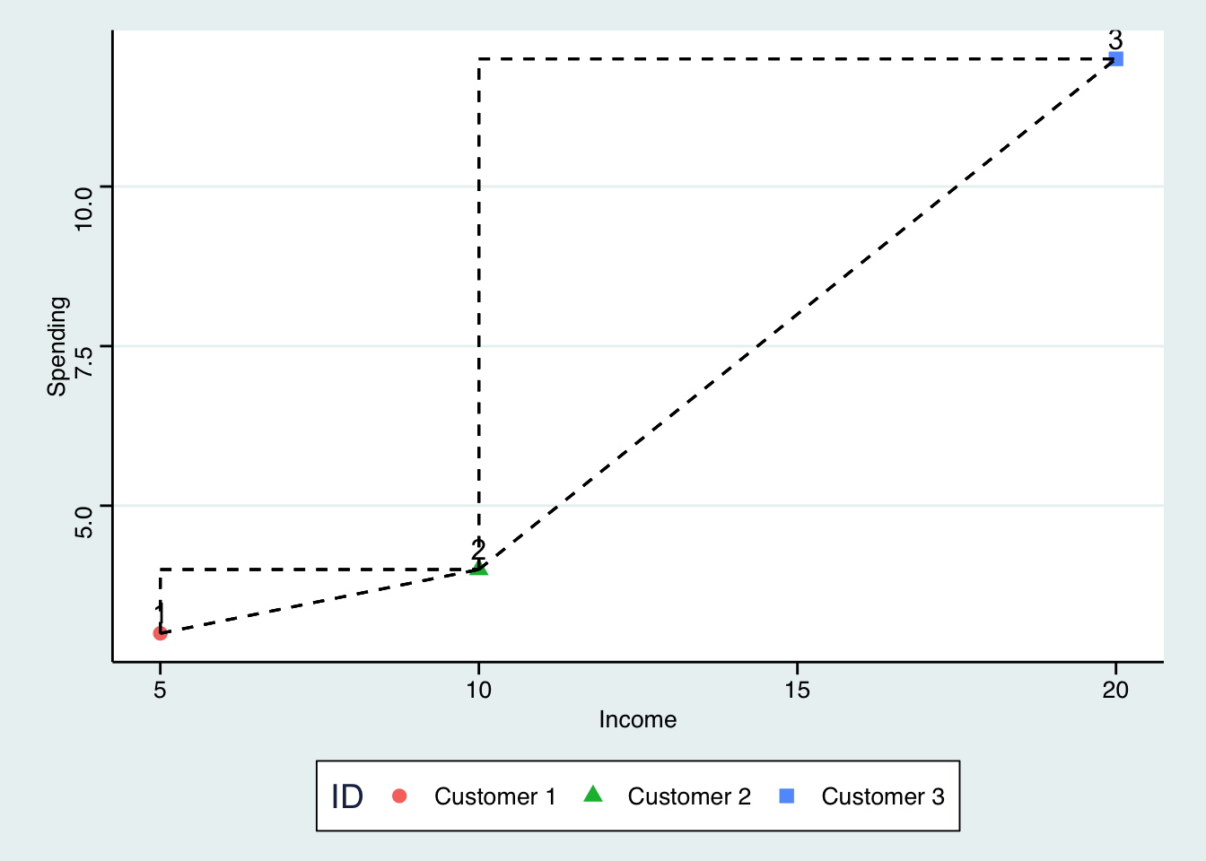
3 Intuition of K-Means Algorithm
3.1 Interactive Illustration of K-Means Clustering
- Download the R Shiny app code from Moodle and let’s run it locally.1

3.2 K-Means Clustering: Step 1

Raw data points; each dot is a customer
The X and Y axes are customer characteristics, for example, income and spending
Obviously, there should be two segments
Let’s see how K-means uses a data-driven approach to classify customers into two segments
3.3 K-Means Clustering: Step 2

We specify two segments
K-means initialises the process by randomly selecting two centroids
Warning
Due to this randomness, different starting points may yield varying results. We need to reinitialise the process repeatedly to ensure robustness of the results. That’s why we set nstart to a value greater than 1 when applying K-means in R.
3.4 K-Means Clustering: Step 3

K-means computes the distance of each customer to the red and blue centroids
K-means assigns each customer to the red or blue segment based on which centroid is closer
3.5 K-Means Clustering: Step 4

K-means updates the centroids of each segment
The red cross and blue cross in the picture are the new centroids
We still see some outliers, so the algorithm continues
3.6 K-Means Clustering: Step 5

K-means computes the distance of each customer to the red and blue centroids
K-means assigns each customer to the red or blue segment based on which centroid is closer
Now the outliers are correctly assigned to each segment
3.7 K-Means Clustering: Step 6

K-means updates the centroids from the previous clustering
K-means computes the distance of each customer to the new centroids
K-means finds that all customers are correctly assigned to their nearest centroids, so the algorithm does not need to continue
We say the algorithm has converged, and it stops
3.8 After-Class Readings
- More technical details: K-means Cluster Analysis