R Basics

Author

Affiliation

Dr Wei Miao

UCL School of Management

1 Hello R

1.1 Bilingual arrangements at MSc Marketing Science

• Primary language is Python

  • Programming (Term 1), Economics and Machine Learning (Term 2)

• Secondary language is R

  • Marketing Analytics and Statistics (Term 1)

1.2 A brief history of R

• R project was initiated by Robert Gentleman and Ross Ihaka (University of Auckland) in 1991; both are statisticians, who later made the language open-source.

• Since 1997, R has been developed by the R Core Team; released versions of R, along with thousands of contributed packages, are distributed through CRAN, the Comprehensive R Archive Network.

• As of July 2026, CRAN hosts 24,455 contributed packages.

• As of July 2026, R is ranked 9th in the TIOBE index¹.

1.3 Why R?

• Highly powerful data analytics and visualizations, including²

  • Data wrangling (dplyr) and data visualization (ggplot)

  • Statistics and Econometrics (major advantage of R over Python)

  • Predictive analytics such as machine learning

• Write beautiful reports, dissertations, presentations using Quarto

  • Write your MSc dissertation

  • Effortlessly build websites. I built and maintain my personal website and the marketing course website all in R.

1.4 One-to-one comparison with Python

• As you will be learning Python in the programming course, it’s good to know the differences between R and Python. The table below gives a general comparison.

• It’s highly recommended that when you learn both languages at the same time, you should be able to compare them side-by-side often.

R versus Python

	R	Python
Language purpose	R is a statistical language specialized in data analytics and visualization. Best for data science, may not be robust for production environments.	Python is a general-purpose language used for the deployment and development of various projects. Best for production environments.
Data analytics	R is better at statistical models and econometrics.	Python is better at machine learning due to support from PyTorch and TensorFlow.
IDEs (Integrated Development Environment)	RStudio	Many options such as Jupyter Notebook, Spyder, PyCharm, etc.
Targeted users	Primary users of R include data scientists and researchers in academia, who heavily rely on data analysis and visualization.	Primary users of Python include developers and programmers.

1.5 A first look at the RStudio Interface

R is the programming language, and we need a “place” to write code. This place is called an Integrated Development Environment (IDE).

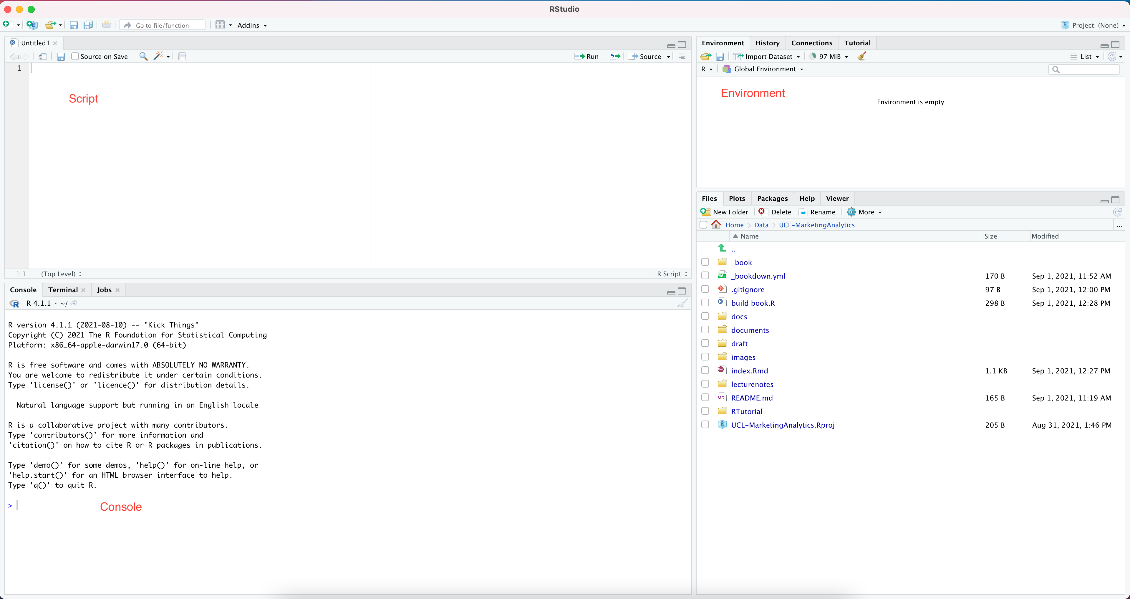
RStudio is the best R IDE. Its interface consists of the following major panels (clockwise from top left):

• script: (top left) where you do the coding

• environment: (top right) a list of named objects that we have generated

• history: (top right) a list of past commands

• help: (bottom right) documentation for functions available in R

• packages: (bottom right) a list of installed packages and tools to manage them

• console: (bottom left) where you can run commands interactively with R and see code outputs

1.6 Where to write R code (I): Console

• You can write code interactively in the R console. See an example: Type the following code into your console and see what happens.

print("Hello World")

[1] "Hello World"

• Used mainly for simple, exploratory, unstructured tasks where you don’t need to keep a record of code.

  • e.g., summary statistics; checking variable values, etc.

1.7 Where to write R code (II): .qmd script

• Quarto³ markdown files have a .qmd suffix. You can think of Quarto as Microsoft Word that can run R code.

• Quarto can create dynamic content with R (it also supports Python, Julia, and more), conveniently combining data analytics work with beautiful reporting.

• Now, let’s create a new Quarto file together! Name it “MyFirstWeekatUCL.qmd” and save it to your Downloads folder.

1.8 Where to write R code (III): .R script

• You can also write R code in an .R script, i.e., a plain text file with a .R suffix.

  • All content in an .R script will be treated as R code and executed when the script is run.

  • If we want to include plain text in an .R script, we must use # to comment out the text.

• .R scripts are more suitable for complex tasks, such as developing an R package.

• However, as data scientists, we should focus more on applying R packages to solve real-world problems rather than developing new ones. Thus, .qmd is the preferred way to write R code in this course.

2 Introduction to Quarto

2.1 YAML header

• You can think of the YAML header as an MS Word-style format template that determines how your final report looks (font family, font size, colour, margins, whether to have a table of contents, whether to number sections, etc.).

• The YAML header is always at the beginning of the .qmd file, separated from the main text by a pair of three dashes (---).

• Quarto reads the YAML header automatically. The --- delimiters and the raw key: value lines never appear in the final report, but fields such as title, subtitle, author, date, and abstract are rendered as the title block you can see at the top of this page.

2.2 Authoring with normal text

RStudio provides two ways to edit a Quarto file: (1) Visual mode and (2) Source mode.

• RStudio’s Visual Editor offers a Microsoft Word-like experience for writing R code and reports.

  • Explore the rich formatting tools available for report authoring.

• If you are familiar with Markdown syntax, you can use Source mode to write the report (optional; for advanced users only).

Visual Mode versus Source Mode

NoteExercise

Create a new Quarto file from RStudio with the following level-1 and level-2 headers:

Level 1: The induction week is fun!

Body: I have met many new friends in the induction week! Can I find my soulmate too?

Level 2: R Basics Tutorial on Friday

Body: OMG, R is so fun to learn! I start to believe that R is the best language in the world!

2.3 Coding with code blocks

• In .qmd files, we write R code in so-called code chunks (sometimes code cells or code blocks) identified with {r}.

• To insert a code chunk, click Insert -> Code Chunk -> R. You can also use the shortcut Ctrl + Alt + I or Cmd + Option + I.

WarningCaveat

Ensure the first line remains {r} only and do not include any comments or code on this line.

• You can run each code chunk interactively by clicking the green solid triangle (run current code chunk). RStudio executes the code in the code chunk and displays the results inline in the source editor, immediately beneath the chunk.

  • Behind the scenes, RStudio sends the code to the R session, but the output is shown inline rather than in the Console. If you prefer the results in the Console instead, choose Chunk Output in Console from the gear menu next to the Render button.

• See an example and try it out on your computer!

print("R is the Best Language! Way better than Python! The battle is on!")

[1] "R is the Best Language! Way better than Python! The battle is on!"

NoteExercise

Insert the above R code block in your Quarto file at the end.

2.4 Rendering a report

When you are done with the coding and report writing, click the Render button in the RStudio IDE to render the file. The rendered report will be in the same folder as your .qmd file.

NoteExercise

Render your Quarto file into a document and see how it looks.

2.5 More learning resources for Quarto (after class)

• The available YAML fields vary based on document format

  • Here for YAML fields for PDF documents

  • Here for MS Word

  • Here for HTML documents

• Markdown syntax

  • Markdown basics

  • Markdown practice

• Quarto (recommended to be reviewed after-class)

  • Get started

3 Basics of R

3.1 Named objects

• R by design uses a mixture of functional programming and object-oriented programming (OOP) paradigms. We will primarily work with objects.

• We use the left arrow <- to create a named object. The keyboard shortcut for <- for Windows users is Alt + -, and for MacOS users, Option + -.

• The <- is an assignment (sometimes referred to as binding) operator, which assigns (binds) the R object on the RHS to the name on the LHS.

• The code below creates a new R object in the memory, which is the number 3, and assigns it to the name x.

# create a number 3 and assign it to the name x
x <- 3

• After an object is created and assigned a name, we can refer to the object by its name.

# print out the value of x
x

[1] 3

• We can also perform operations on the object

# Question: hmmm, why does Wei choose these two numbers?
x^2

[1] 9

x^3

[1] 27

NoteExercise

Insert a code block in your Quarto file, which does the following:

• Create an object with name ‘x’ with the formula of 2 + 2

3.2 Rules for naming objects

For a variable name to be valid, it should follow these rules:

• It should contain letters, numbers, and only the dot . or underscore _ characters as separators (spaces are not allowed).

• It cannot start with a number (e.g., 2iota). It may start with a dot if the dot is not followed by a number (e.g., .hiddenVar), but leading dots are typically used for hidden objects.

# 2iota <- 2
# .2iota <- 2

• R does allow us to reuse common function names (e.g., mean, sum) as object names; doing so merely masks the function and will confuse us later, so avoid it.

• Reserved words (e.g., if, else, for, TRUE, FALSE, NULL, NA) cannot be used as object names at all: R raises an error.

# mean <- 2  # avoid masking built-in functions

TipSome good practices for naming objects

• Use meaningful, memorable names to name an object. For instance, use prefix df_ or data_ to name datasets. Use prefix vec_ to name vectors.

• Use consistent naming conventions, such as snake_case or camelCase.

3.3 Functions

• A function takes one or several R objects as input arguments,⁴ performs specific operations on them, and then returns an output.

• For instance, an R’s built-in function sqrt() takes a number as input, and returns the square root of the number. Let’s use it on object x.

sqrt(x)

[1] 1.732051

• To learn how to use a new function, search the function by its name in RStudio’s help panel, or type ?function_name in the console.

?sqrt

• Data analytics is all about taking various datasets as inputs, running operations (data cleaning, data transformation, data visualization, etc.) on the datasets, and then generating business insights. Therefore, functions are the building blocks of data analytics.

NoteExercise

1. Search and learn the usage of function “log()”.
2. Insert a code block in your Quarto file to compute the logarithm of x.

3.4 Packages: Collection of ready-to-use functions

The base R already includes many useful functions to perform basic tasks, but as data scientists, we need more.

To perform certain tasks (such as training a machine learning model), we can definitely write our own code from scratch, but it takes lots of (unnecessary) effort. Fortunately, many packages have been written by others for us to directly use.

• To download a package, hit Tools -> Install Packages in RStudio, and type the package name in the pop-up window. Now, download the package praise.

• To load the packages, we need to type library().

library(praise)

• Now that the package is loaded, you can use the functions in it. praise() is a function in the praise package.

praise()

[1] "You are tiptop!"

TipTips

• Packages need to be downloaded only once, but must be loaded in each new RStudio session.

3.5 Comment codes

You can put a # before any code to indicate that any text after the # on the same line is your comment, and will not be run by R.

It’s good practice to comment your code often, so that future-you can remember what you were trying to achieve.

# print("Let's fund Wei for an iPhone 17 Pro Max as a birthday gift!")

# Is x 1 or 2 below?
x <- 1 # +1

4 Basic Data Type Classes in R

Because R is object-oriented, we will work on objects most of the time.

In OOP technical terms, the type of an object is called its class.

Think of a class as a blueprint for an object. This blueprint defines the object’s properties and what R can do with it.

For example, the blueprint for a numeric object specifies that you can perform mathematical calculations on it, while the blueprint for a character object does not.

4.1 Basic data type classes

4.1.1 Numeric

• We can use R as a calculator for numeric objects

# Numeric Vector
num2 <- 2.5
log(num2)

[1] 0.9162907

num2^2

[1] 6.25

exp(num2)

[1] 12.18249

4.1.2 Logical (TRUE, FALSE)

• Logical objects are used to store logical values, such as TRUE and FALSE.

num2 <- 2.5

# larger than 2?
num2 > 2

[1] TRUE

# smaller than 2?
num2 < 2

[1] FALSE

# equal to 2?
num2 == 2

[1] FALSE

# not equal to 2?
num2 != 2

[1] TRUE

• Sometimes, we may need to run multiple relational operations. We can use logical operators to combine multiple relational operations.

TRUE & FALSE # and

[1] FALSE

TRUE | FALSE # or

[1] TRUE

!TRUE # not

[1] FALSE

• For instance, we may want to know if a number is between 3 and 8.

num2 >= 3 & num2 <= 8

[1] FALSE

4.1.3 Character

• Characters are enclosed within a pair of quotation marks.

• Single or double quotation marks can both work in R.

• Even if a character may contain numbers, it will be treated as a character, and R will not perform any mathematical operations on it.

str1 <- "1 + 1 = 2"

# Can the following code run?
# str1 > 1

• Yes, it runs and returns TRUE. > is a relational operator, not an arithmetic one: R coerces the number 1 to the character "1" and compares the two as text.

• That is also why "10" > 9 is FALSE: as text, "10" comes before "9".

• Arithmetic on a character vector, by contrast, does throw an error, as we will see in the Class conversion section below.

4.2 Check object class using class()

We can use class() to check the type of an object in R.

a <- "1+1"
class(a)

[1] "character"

b <- 1 + 1
class(b)

[1] "numeric"

c <- 3^2 > 5
class(c)

[1] "logical"

This is very useful when we first load data from external databases; we need to make sure variables are of the correct data types.

4.3 Class conversion

Sometimes, the class of variables from raw data may not be what we want; we need to change the class of a variable to the appropriate one.

See the following example:

• a is a string, and we cannot use mathematical operations on it, or R will report errors.

a <- "1"
class(a)

[1] "character"

a + 1

Error in `a + 1`:
! non-numeric argument to binary operator

• We can convert a to a numeric value. To convert from character to numeric, we use as.numeric()

a <- "1"
a <- as.numeric(a)
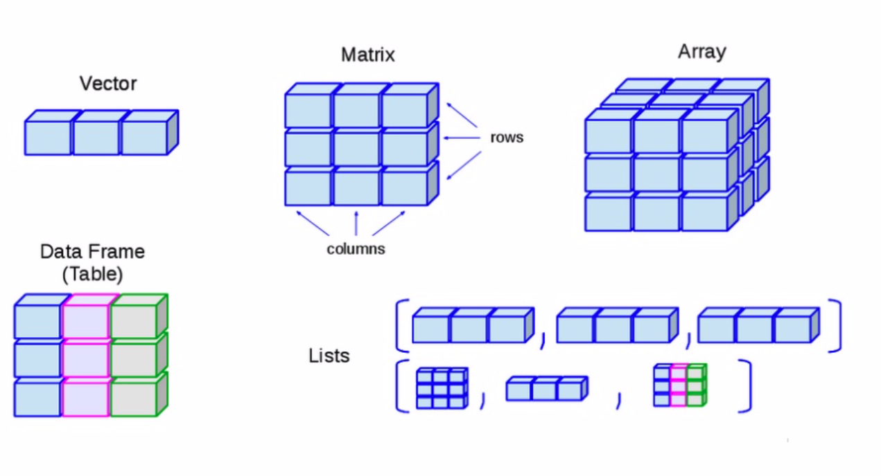
class(a)

[1] "numeric"

a + 1

[1] 2

5 Vectors

Next, we will learn about data structures in R. You can think of data structures as containers that store data.

Below is the complete list of data structures in R.

.

We will learn the basics of vectors and matrices in this tutorial.

5.1 Creating vectors

5.1.1 Creating vectors: c()

• In R, a vector is a collection of elements of the same data class, often used to store a variable of a dataset. For instance, a vector can store the income of a group of people, the final grades of students, etc.

• A vector can be created using the function c() by listing all the values in the parentheses, separated by commas ,.

• c() stands for “combine”.

Income <- c(1, 3, 5, 10)
Income

[1]  1  3  5 10

• The class of a vector is the class of the elements in the vector.

class(Income)

[1] "numeric"

• Vectors must contain elements of the same class. If they do not, R will automatically coerce all elements to a common type according to coercion rules (e.g., if any element is character, the result is character).

x <- c(1, "intro", TRUE)
class(x)

[1] "character"

5.1.2 Checking the number of elements in a vector: length()

You can count the number of elements in a vector using the command length()

x <- c("R", " is", " the", " best", " language")
length(x)

[1] 5

5.1.3 Creating numeric sequences: seq()

It is also possible to easily create sequences with patterns

• Use seq() to create a sequence with fixed steps

# use seq()
seq(from = 1, to = 2, by = 0.1)

 [1] 1.0 1.1 1.2 1.3 1.4 1.5 1.6 1.7 1.8 1.9 2.0

• If the step is 1, there’s a convenient way using start_integer:end_integer

2:5

[1] 2 3 4 5

5.1.4 Combine multiple vectors into a single vector: c()

• Sometimes, we may want to combine multiple vectors into one. For instance, we may have collected income data from two different sources, and we want to combine them into one vector.

• We can use c() to combine different vectors; this is very commonly used to combine vectors.

Income_source1 <- 1:3
Income_source2 <- c(10, 15)

Income_all <- c(Income_source1, Income_source2)

NoteExercise

Create a sequence of {1,1,2,2,3,3,3}.

5.2 Indexing and subsetting

We put the index of elements we would like to extract in a square bracket [ ].

# create a vector of monthly salaries for 4 lecturers at UCL

income <- c(5000, 5500, 6000, 9000)

• Extract a single element: use the index of the element

# what is the income of the 3rd lecturer?
income[3]

[1] 6000

• Extract multiple elements: use a vector of indices

# what are the incomes of the 1st, 3rd, and 4th lecturers?
income[c(1, 3, 4)]

[1] 5000 6000 9000

5.3 Element-wise arithmetic operations

R is a vectorised language, which broadcasts operations to all elements in a vector. This behaviour is also called element-wise operations, or broadcasting.

• If you perform mathematical operations on a numeric vector with only a single number, the operation will be applied to all elements in the original vector.

# create a vector of numbers
x <- c(1, 3, 8, 7)

# add 2 to the vector x
x + 2

[1]  3  5 10  9

# You will see that 2 is added to each element in the vector x

# similar rules apply to other arithmetic operations
x * 2

[1]  2  6 16 14

NoteExercise

Create the geometric sequence {2, 4, 8, 16, 32} using what we learned so far.

5.4 Element-wise relational operations

• Besides arithmetic operations, we can also perform relational operations on vectors.

x <- c(1, 3, 8, 7)
x > 2

[1] FALSE  TRUE  TRUE  TRUE

• We can also compare a vector with another vector, because R is vectorized

incomeUCL <- c(6000, 4600, 7000, 9100, 10000)
incomeImperial <- c(5000, 4500, 6000, 9000, 10000)
incomeUCL > incomeImperial

[1]  TRUE  TRUE  TRUE  TRUE FALSE

5.5 Special relational operation: %in%

• A special relational operation is %in% in R, which tests whether an element exists in the object.

x <- c(1, 3, 8, 7)

3 %in% x

[1] TRUE

2 %in% x

[1] FALSE

5.6 After-class exercise

1. Create a vector of 10 numbers from 1 to 10, and extract the 2nd, 4th, and 6th elements.

2. Create a vector of 5 numbers from 1 to 5, and check if 3 is in the vector.

3. Now the interest rate is 0.1, and you have 1000 pounds in your bank account. Calculate the amount in your bank account after 1 year, 2 years, and 3 years, respectively.

6 Matrices

6.1 Matrices: creating matrices

6.1.1 Creating matrices: matrix()

• A matrix can be created using the command matrix()
  • the first argument is the vector to be converted into a matrix
  • the second argument is the number of rows
  • the third argument is the number of columns

matrix(1:9, nrow = 3, ncol = 3)

     [,1] [,2] [,3]
[1,]    1    4    7
[2,]    2    5    8
[3,]    3    6    9

Important

R by default inserts elements vertically by columns.

• R will fill in the matrix by column and discards any extra elements, with a warning message

matrix(1:9, nrow = 3, ncol = 2)

Warning in matrix(1:9, nrow = 3, ncol = 2): data length [9] is not a
sub-multiple or multiple of the number of columns [2]

     [,1] [,2]
[1,]    1    4
[2,]    2    5
[3,]    3    6

6.1.2 Creating matrices: inserting by row

However, we can ask R to insert by rows by setting the byrow argument.

matrix(1:9, nrow = 3, ncol = 3, byrow = TRUE)

     [,1] [,2] [,3]
[1,]    1    2    3
[2,]    4    5    6
[3,]    7    8    9

6.1.3 Creating matrices: concatenate matrices cbind() and rbind()

We can use cbind() and rbind() to concatenate vectors and matrices into new matrices.

• cbind() does the column binding

a <- matrix(1:6, nrow = 2, ncol = 3)

a

     [,1] [,2] [,3]
[1,]    1    3    5
[2,]    2    4    6

cbind(a, a) # column bind

     [,1] [,2] [,3] [,4] [,5] [,6]
[1,]    1    3    5    1    3    5
[2,]    2    4    6    2    4    6

• rbind() does the row binding

rbind(a, a) # row bind

     [,1] [,2] [,3]
[1,]    1    3    5
[2,]    2    4    6
[3,]    1    3    5
[4,]    2    4    6

6.2 Matrices: indexing and subsetting

Matrices have two dimensions: rows and columns. Therefore, to extract elements from a matrix, we specify which row(s) and which column(s) we want.

x <- matrix(1:9, nrow = 3, ncol = 3)
x

     [,1] [,2] [,3]
[1,]    1    4    7
[2,]    2    5    8
[3,]    3    6    9

• Extract the element in the 2nd row, 3rd column.
  • Use square brackets with a comma inside [ , ] to indicate subsetting; the argument before the comma is the row index, and the argument after the comma is the column index.
    • 2 is the row index, so we extract from the second row.
    • 3 is the column index, so we extract from the third column.
    • Altogether, we extract the single element in row 2, column 3.

x[2, 3] # the element in the 2nd row, 3rd column

[1] 8

• If we leave a dimension blank, we extract all elements along that dimension.
  • If we want to take out the entire first row
    • 1 is specified for the row index
    • column index is blank

x[1, ] # all elements in the first row

[1] 1 4 7

NoteExercise

1. Extract all elements in the second column

2. Extract all elements in the first and third rows

6.3 Matrices: operations

6.3.1 Apply a math function to a matrix

Let’s use 3 matrices x, y, and z:

x <- matrix(1:6, nrow = 3)
y <- matrix(1:6, byrow = T, nrow = 2)
x

     [,1] [,2]
[1,]    1    4
[2,]    2    5
[3,]    3    6

y

     [,1] [,2] [,3]
[1,]    1    2    3
[2,]    4    5    6

• Functions will be vectorized over all elements in a matrix

z <- x^2
z

     [,1] [,2]
[1,]    1   16
[2,]    4   25
[3,]    9   36

6.3.2 Matrices’ operations: matrix addition and multiplication

• If the two matrices are of the same dimensions, they can do element-wise operations, including element-wise addition and element-wise multiplication

x + z # elementwise addition

     [,1] [,2]
[1,]    2   20
[2,]    6   30
[3,]   12   42

x * x

     [,1] [,2]
[1,]    1   16
[2,]    4   25
[3,]    9   36

• If we want to perform the matrix multiplication as in linear algebra, we need to use %*%
  • x and y must have conforming dimensions

x

     [,1] [,2]
[1,]    1    4
[2,]    2    5
[3,]    3    6

y

     [,1] [,2] [,3]
[1,]    1    2    3
[2,]    4    5    6

x %*% y # matrix multiplication

     [,1] [,2] [,3]
[1,]   17   22   27
[2,]   22   29   36
[3,]   27   36   45

6.3.3 Matrices’ operations: inverse and transpose

• We use t() to do matrix transpose

x

     [,1] [,2]
[1,]    1    4
[2,]    2    5
[3,]    3    6

t(x) # transpose

     [,1] [,2] [,3]
[1,]    1    2    3
[2,]    4    5    6

• We use solve() to get the inverse of a matrix (the input must be square and non-singular)

x

     [,1] [,2]
[1,]    1    4
[2,]    2    5
[3,]    3    6

solve(t(x) %*% x) # inverse; must be on a square, non-singular matrix

           [,1]       [,2]
[1,]  1.4259259 -0.5925926
[2,] -0.5925926  0.2592593

7 Data Frames

7.1 Data frames: creating data.frame

7.1.1 Data frames: create dataframe using data.frame()

• You can think of a data.frame as a spreadsheet in Excel.

df <- data.frame(
    id = 1:4,
    name = c("Dimitri", "Tjun", "Anil", "Wei"),
    wage = rnorm(n = 4, mean = 10^5, sd = 10^3),
    male = c(TRUE, TRUE, TRUE, TRUE)
)
df

• Data frames can also be created from external sources, e.g., from a CSV file or a database.

7.2 Data frames: basics

• Each row stands for an observation; each column represents a variable.

• Each variable should have a unique name.

• Each column must contain a single data type, but different columns can store different data types.

  • Compare with matrix?

• Each column must be the same length, because rows have the same length across variables.

7.3 Data frames: check dimensions and variable types

• You can verify the size of the data.frame using the command dim(); or nrow() and ncol()

nrow(df)

[1] 4

ncol(df)

[1] 4

• You can get the data type info using the command str()

str(df)

'data.frame':   4 obs. of  4 variables:
 $ id  : int  1 2 3 4
 $ name: chr  "Dimitri" "Tjun" "Anil" "Wei"
 $ wage: num  99533 99733 101366 99313
 $ male: logi  TRUE TRUE TRUE TRUE

• Get the variable names of the data frame

names(df)

[1] "id"   "name" "wage" "male"

8 Other Data Structures (Optional)

8.1 Arrays

• We can use array() to generate a high-dimensional array

• Just like vectors and matrices, arrays can include only data types of the same kind.

• A 3D array is basically a combination of matrices each laid on top of other

x <- 1:4
x <- array(data = x, dim = c(2, 3, 2))
x

, , 1

     [,1] [,2] [,3]
[1,]    1    3    1
[2,]    2    4    2

, , 2

     [,1] [,2] [,3]
[1,]    3    1    3
[2,]    4    2    4

8.2 Lists

A list is an R object that can contain anything. A list is useful when you need to store objects for later use.

x <- 1:2
y <- c("a", "b")
L <- list(numbers = x, letters = y)

8.3 Lists: indexing and subsetting

There are many ways to extract a certain element from a list.

• by index
• by the name of the element
• by dollar sign $

L[[1]] # extract the first element

[1] 1 2

L[["numbers"]] # based on element name

[1] 1 2

L$numbers # extract the element called numbers

[1] 1 2

After extracting the element, we can work on the element further:

L$numbers > 2

[1] FALSE FALSE

9 Programming Basics: Flow Control

9.1 if/else

Sometimes, you may want to run code based on different conditions. For instance, if an observation is a missing value, you might impute it with the population average. This is where if/else comes in.

if (condition == TRUE) {
  action 1
} else if (condition == TRUE ){
  action 2
} else {
  action 3
}

Example 1:

a <- 9

if (a > 10) {
    larger_than_10 <- TRUE
} else {
    larger_than_10 <- FALSE
}

larger_than_10

[1] FALSE

Example 2:

x <- -5
if (x > 0) {
    print("x is a positive number")
} else {
    print("x is not a positive number")
}

[1] "x is not a positive number"

9.2 Loops

As the name suggests, in a loop the program repeats a set of instructions multiple times, until a stopping criterion is met.

Looping is very useful for repetitive jobs.

for (i in 1:10) { # i is the iterator
    # loop body: gets executed each time
    # the value of i changes with each iteration
}

9.3 Nested loops

We can also nest loops inside other loops.

x <- cbind(1:3, 4:6) # column bind
x

     [,1] [,2]
[1,]    1    4
[2,]    2    5
[3,]    3    6

y <- cbind(7:9, 10:12) # column bind
y

     [,1] [,2]
[1,]    7   10
[2,]    8   11
[3,]    9   12

z <- x

for (i in 1:nrow(x)) {
    for (j in 1:ncol(x)) {
        z[i, j] <- x[i, j] + y[i, j]
    }
}

z

     [,1] [,2]
[1,]    8   14
[2,]   10   16
[3,]   12   18

9.4 User-defined functions

A function takes arguments as input, performs some specified actions, and then returns a result.

Functions are very useful. When we would like to test different ideas, we can combine functions with loops: We can write a function which takes different parameters as input, and we can use a loop to go through all the possible combinations of parameters.

9.4.1 User-defined function syntax

Here is how to define a function in general:

function_name <- function(arg1, arg2 = default_value) {
    # write the actions to be done with arg1 and arg2
    # you can have any number of arguments, with or without defaults
    return() # the last line is to return some value
}

Example:

magic <- function(x, y) {
    results <- x^2 + y

    return(results)
}

magic(2, 3)

[1] 7

9.4.2 Arguments

• Default values: A user-defined function (UDF) can have default values for arguments by using arg = default_value. If the user does not provide a value for the argument when calling the UDF, the default value will be used.

magic <- function(x, y = 1) {
    results <- x^2 + y

    return(results)
}

magic(2)

[1] 5

• Missing values: If the user does not provide a value for an argument without a default value, R will throw an error.

magic <- function(x, y) {
    results <- x^2 + y

    return(results)
}

magic(2)

Error in `magic()`:
! argument "y" is missing, with no default

• Argument matching: Positional matching respects the order of arguments. You can also use named arguments to pass values in any order (e.g., magic(y = 3, x = 2)).

magic <- function(y, x) {
    results <- x^2 + y

    return(results)
}

magic(y = 3, x = 2)

[1] 7

9.4.3 Returned value

• We can return a value from a function using the return() function. The value returned can be of any data type.

magic <- function(x, y) {
    result <- x^2 + y

    return(result)
}

magic(2, 3)

[1] 7

• If the function does not have a return() statement, it will return the last value calculated in the function.

magic <- function(x, y) {
    x + y
}

magic(2, 3)

[1] 5

9.5 Variable scope

• Variables created inside a function are local to the function, and cannot be accessed outside the function.

magic <- function(x, y) {
    result <- x^2 + y

    return(result)
}

result

Error:
! object 'result' not found

9.6 A comprehensive example

Task: write a function, which takes a vector as input, and returns the max value of the vector

get_max <- function(input) {
    max_value <- input[1]
    for (i in seq_along(input)[-1]) {
        if (input[i] > max_value) {
            max_value <- input[i]
        }
    }

    return(max_value)
}

get_max(c(-1, 3, 2))

[1] 3

• Always use seq_along() (or seq_len()) to build the iterator of a loop: they return an empty sequence when there is nothing to iterate over, whereas 2:length(input) counts backwards to c(2, 1) for a length-1 input and the loop then breaks.

NoteExercise

Write your own version of which.max() function

Footnotes

1. TIOBE Programming Community index is a measure of programming language popularity. Click here to reach the website.

2. There are many R-exclusive packages, such as the state-of-the-art causal machine learning library grf , which we will learn in the final week.

3. Why the name Quarto? “We wanted to use a name that had meaning in the history of publishing and landed on Quarto, which is the format of a book or pamphlet produced from full sheets printed with eight pages of text, four to a side, then folded twice to produce four leaves. The earliest known European printed book is a Quarto, the Sibyllenbuch, believed to have been printed by Johannes Gutenberg in 1452–53.”

4. Some functions may not take any input arguments. These functions are designed to be used as standalone functions, such as praise().